DISTRIBUTIONS
Beta distribution
The beta distribution is most commonly used as a Bayes distribution to model uncertainty in a parameter p. The density is
![]() for 0 < p< 1
for 0 < p< 1
For most applications the gamma functions in the front can be ignored ¾ they only form a normalizing constant, to ensure that the density integrates to 1. The important feature of the density is that
![]() ,
,
where the symbol µ denotes “is proportional to.” The parameters of the distribution, a and b, must both be positive. The shape of the beta density depends on the size of the two parameters. If a < 1, the exponent of p is negative in equation for the density, and therefore the density is unbounded as p ® 0. Likewise, if b < 1, the density is unbounded as p ® 1. If both a > 1 and b > 1, the density is roughly bell shaped, with a single mode.
The mean and variance of the distribution are
mean, denoted m here, = a/(a + b)
variance = m(1 - m)/(a + b + 1).
The formula for the variance shows that as the sum a + b becomes large, the variance becomes small, and the distribution becomes more tightly concentrated around the mean. Although the moments are algebraic functions of the parameters, the percentiles are not so easily found. RADS finds the percentiles of a beta distribution using rather elaborate numerical calculations.
Two beta distributions are plotted below.
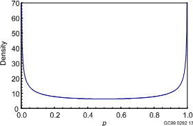
Beta(0.5, 0.5) density. This is the Jeffreys non-informative prior distribution for p.
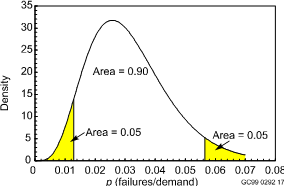
Beta(5.2, 160.1) density, with 5th and 95th percentiles shown. The mean is 5.2/(5.2+160.1) = 0.0315, and the standard deviation is [0.0315(1 - 0.0315)/(5.2 + 160.1 + 1)]1/2 = 0.0135.
The beta distributions form the conjugate family for binomial data. That is, suppose that independent failures and successes are observed, with Pr(failure) = p on each demand. Denote the total number of failures by x and the total number of demands by n. If the prior distribution for p is a beta distribution with parameters aprior and bprior , then the posterior distribution is also a beta distribution, with
aposterior = aprior + x
bposterior = bprior + (n - x) .
This gives an intuitive interpretation for the prior parameters: aprior is to the effective number of failures in the prior information, and bprior is the effective number of successes in the prior information.
RADS allows a beta distribution to be specified by entering any two of a, b, and m. RADS then calculates and displays the third value.
Gamma distribution
The gamma distribution has many uses. An important use in RADS is as a Bayes prior distribution for a frequency l. For this application, the most convenient parameterization is
![]() for
l
> 0 .
for
l
> 0 .
For most applications the terms that do not involve l can be ignored ¾ they only form a normalizing constant, to ensure that the density integrates to 1. The important feature of the density is that
![]()
where the symbol µ denotes “is proportional to.” The parameters of the distribution, a and b, must both be positive.
Some references use other letters for the parameters a and b, and in some applications it is more convenient to parameterize in terms of b¢ = 1/b. The two parameters must both be positive. Here l has units 1/time and q has units of time, so the product lq is unitless. For example, if l is the frequency of events per critical-year, q has units of critical-years. The parameter q corresponds to the scale of l C if we convert l from 1/hours to 1/years by multiplying it by 8760, we correspondingly divide q by 8760, converting it from hours to years. The other parameter, a, is unitless, and is called the shape parameter. The gamma function, G(a), is a standard mathematical function; if a is a positive integer, G(a) equals (a!1)!
The shape of the gamma density depends on the first parameter. If a < 1, the exponent of l is negative in the equation for the density, and therefore the density is unbounded as l ® 0. If a > 1, the density is roughly bell shaped (though skewed to the right), with a single mode. As a ® ¥, the density becomes symmetrical around the mean.
The mean and variance of the distribution are
mean = a/q
variance = a/q2 .
Note that the units are correct, units 1/time for the mean and 1/time2 for the variance. The percentiles of the gamma distribution are calculated by RADS using numerical algorithms. A typical gamma density is plotted below.
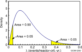
Gamma density with a = 2.53 and b = 15.52 reactor-critical-years. The 5th and 95th percentiles are also shown.
The gamma distributions form a conjugate family for Poisson data. That is, suppose that events occur independently of each other in time, with Pr(an event occurs in time interval of length Dt) » lDt. Let x be the number of events observed in a time period of length t. If l has a gamma prior distribution with parameters aprior and bprior , then the posterior distribution is also a gamma distribution, with
aposterior = aprior + x
bposterior = bprior + t .
This gives an intuitive interpretation for the prior parameters: aprior is to the effective number of events in the prior information, and bprior is the corresponding effective time period in the prior information.
One “distribution” that is often used is the Jeffreys non-informative prior, defined for events in time as a gamma(0.5, 0) distribution. In fact, this is not a distribution, because the second parameter is not positive. Ignoring that problem and taking the limit of a gamma(a, b) density as b ® 0, the density is seen to be proportional to
![]() .
.
This function does not have a finite integral. Therefore, it is not a density, and cannot be made into a density by multiplication by some suitable normalizing constant. It is called an “improper distribution.” Nevertheless, it may be treated as a density in formal algebraic calculations given above, yielding
aposterior = aprior + x = x + 0.5
bposterior = bprior + t = t + 0 = t .
The Jeffreys non-informative prior distribution is plotted below.
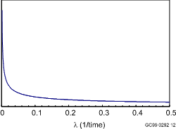
Jeffreys non-informative prior distribution for l, defined as l-1/2 .
RADS allows a gamma distribution to be specified by ???
Normal distribution
The normal distribution is not used directly by RADS, but it is used indirectly, in calculations with the lognormal or logistic-normal distributions.
X is normally distributed with mean m and variance s2 if its density is of the form
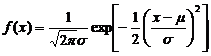 .
.
The parameter m can have any value, and the parameter s must be positive. This density is positive for all x, positive and negative. That is, a normally distributed random variable can take any value, positive or negative.
The mean of the distribution is m and the variance is s2 . Percentiles or probabilities involving X can be found from a table of the standard normal distribution, that is, the normal distribution with mean 0 and variance 1. This is done using the following fact. If X has a normal(m, s2) distribution, then (X - m)/s has a normal(0, 1) distribution. For example, suppose that X is normal with m = -3.4 and m and s = 1.2, and the 95th percentile of X is needed. This is the number a such that Pr(X £ a) = 0.95. The desired number is found by solving
0.95 = Pr(X £ a)
Pr[(X - m)/s £ (a - m)/s ] performing the same algebra on both sides of the inequality
Pr[Z £ (a - m)/s] denoting (X - m)/s by Z, where Z is normal(0, 1)
Therefore, (a - m)/s must equal 1.645, because a table of the standard normal distribution shows that 1.645 is the 95th percentile of the distribution. Algebraic rearrangement then shows that
a = m + 1.645s .
Lognormal distribution
Y has a lognormal distribution if ln(Y) has a normal distribution. For use in formulas, denote ln(Y) by X here. Then Y = exp(X). X can take all real values, implying that Y can take all positive values. In Bayesian estimation, an event frequency, l, is sometimes given a lognormal prior distribution. A probability of failure, p, is also sometimes assigned a lognormal prior distribution, even though a lognormal variable can take all possible positive values and p must be £ 1. This conflict is of negligible importance if the lognormal distribution assigns almost all the probability to the interval from 0 to 1.
Let Y be lognormally distributed. That is X = ln(Y) has a normal(m, s2) distribution. The density of Y satisfies
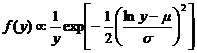 .
.
It is important to note that this is not simply the normal density with lny substituted for x. A 1/y term is also present that does not correspond to anything in the normal density. [The 1/y term enters when (1/y)dy is used to replace dx, similar to the change-of-variables rule in calculus.]
The mean and variance of Y are
mean = exp(m + s2/2)
variance = exp(2m + s2)[exp(s2) - 1] .
The percentiles are obtained by direct translation from the normal distribution: qth percentile of Y = exp(qth percentile of X). In particular
median = exp(m)
95th percentile = exp(m + 1.645s)
5th percentile = exp(m - 1.645s) .
It follows that the error factor, defined as the ratio of the 95th percentile to the median, is
EF = exp(1.645s) .
RADS allows a lognormal distribution to be specified in several ways, according to which pair of inputs the user chooses to enter: either m and s, or the mean and error factor, or the median and error factor. Any of these pairs uniquely determines the distribution. RADS then calculates and displays the other values.
Logistic-normal distribution
The distribution of p has a logistic-normal distribution if ln[p/(1 - p)] has a normal distribution. The function ln[p/(1 - p)] is called the logit function of p. For use in formulas, denote ln[p/(1 - p)] by X here. Then p = exp(X)[1 + exp(X)]. X can take all real values, implying that p can take all values between 0 and 1. This makes the logistic-normal a natural prior distribution for a probability p, although it has not been widely used in PRA applications. If p is small with high probability, the term (1 - p) is usually close to 1, and logit(p) is usually close to ln(p). Therefore, the logistic-normal and lognormal distributions are nearly the same, unless p can take relatively large values (say 0.1 or larger) with noticeable probability.
The moments of the logistic-normal distribution apparently are not given by simple formulas. The percentiles, on the other hand, are obtained by direct translation from the normal distribution: qth percentile of p = exp(qth percentile of X)/{1 + exp(qth percentile of X)]. In particular
median = exp(m)/[1 + exp(m)]
95th percentile = exp(m + 1.645s)/[1 + exp(m + 1.645s)]
RADS allows a logistic-normal distribution to be specified in two ways, according to which pair of inputs the user chooses to enter: either m and s, or the median and 95th percentile. Either of these pairs uniquely determines the distribution. RADS then calculates and displays the other values.
Binomial distribution
The standard model for failures on demand assumes that the number of failures has a binomial distribution. The following assumptions lead to this distribution.
1. Each demand is a failure with some probability p, and is a success with probability 1 ! p.
2. Occurrences of failures for different demands are statistically independent; that is, the probability of a failure on one demand is not affected by what happens on other demands.
Under these assumptions, the number of failures, X, in some fixed number of demands, n, has a binomial(n, p) distribution,
![]()
where
![]() .
.
This distribution has two parameters, n and p, of which only the second is treated as unknown by RADS. The mean of the binomial(n, p) distribution is np, and the variance is np(1 - p).
Assumption 1 says that the probability of failure on demand is the same for every demand. If data are collected over a long time period, the assumption requires that the failure probability does not change or (less realistically) that the analyst does not care if it changes because only the average probability of failure on a random demand is needed. Likewise, if the data are collected from various plants, the assumption is that p is the same at all plants, or that the analyst does not care about between-plant differences but only about the industry average.
Assumption 2 says that the outcome of one demand does not influence the outcomes of later demands. Presumably, events at one plant have little effect on events at a different plant. However, the experience of one failure might cause a change in procedures or design that reduces the failure probability on later demands at the same plant. The binomial distribution assumes that such effects are negligible.
RADS tries to check the data for violations of the assumptions. Thus, it looks for differences between plants or over time. If variation is seen between plant or between systems, RADS allows for a more general model, the empirical Bayes model. If variation is seen over time, RADS allows for modeling of a trend in p.
Poisson distribution
The standard model for events in time assumes that the event count has a Poisson distribution. The following assumptions lead to this distribution.
1. The probability that an event will occur in any specified short exposure time period is approximately proportional to the length of the time period. In other words, for an interval of length Dt the probability of an occurrence in the interval is approximately l H Dt for some l > 0.
2. Exactly simultaneous events do not occur.
3. Occurrences of events in disjoint exposure time periods are statistically independent.
Under the above assumptions, the number of occurrences X in some fixed exposure time t is a Poisson distributed random variable with mean m = lt,
![]() for x = 0, 1, 2, …
for x = 0, 1, 2, …
The parameter l is a rate or frequency. To make things clearer, the kind of event is often stated, that is, “initiating event rate” or “very-small-LOCA frequency.” Because the count of events during a fixed period is a unitless quantity, the mean number of occurrences m is also unitless. However, the rate l depends on the units for measuring time. In other words, the units of l are 1 per unit of time, such as 1/reactor-year or 1/component-hr.
This model is called a Poisson process. It is extremely simple, because it is completely specified by the exposure time, t, and the one unknown parameter, l. Assumption 1 implies that the rate l does not change, neither with a monotonic trend, nor cyclically, nor in any other way. Assumption 2 says that exactly simultaneous events do not occur. The only way that they could occur (other than by incredible coincidence) is if some synchronizing mechanism exists, a common cause. Therefore, the operational interpretation of Assumption 2 is that common-cause events do not occur. Assumption 3 says that the past history does not affect the present. In particular, occurrence of an event yesterday does not make the probability of another event tomorrow either more or less likely. This says that the events do not tend to occur too much in clusters, nor do they tend to be systematically spaced and evenly separated.
RADS tries to check the data for violations of the assumptions. Thus, it looks for differences between plants or over time. If variation is seen between plant or between systems, RADS allows for a more general model, the empirical Bayes model. If variation is seen over time, RADS allows for modeling of a trend in l.
The mean and variance of a Poisson(m) distribution are both equal to m.