Reliability Calculator
The U. S. Nuclear Regulatory Commission (NRC) in conjunction with the Idaho National Laboratory (INL) developed software to evaluate data for use in Probabilistic Risk Assessments (PRA).
The software uses US commercial nuclear power plant data and statistical routines to provide statistical analysis of the data.
The Reliability Calculator uses these statistical routines to allow risk analysts to statistically analyze their own data and is available to the public.
The Reliability Calculator analyzes two basic types of data; ‘Un-partitioned Data’ and ‘Partitioned Data’.
- Un-partitioned Data is data that the analyst only knows the total failures (events) and total demands (run hours).
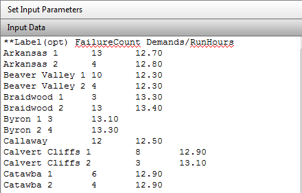
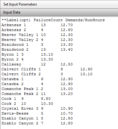
- Partitioned Data is data that has been kept at some level of detail and should consist of a list of pairs of failures (events) and demands (run hours). These pairs can be rolled up from more detailed data—as in trending data which would be a pair summed over the year.
Analysis of Un-partitioned Data
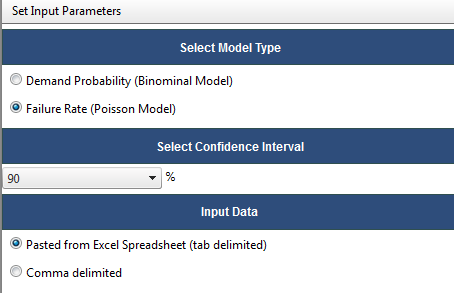
Two types of un-partitioned analyses are provided: Classical and Bayesian Update.
Calculate Classical
Demand. Suppose that similar components or systems are repeatedly demanded, that the success or failure on any demand is independent of the outcomes on other demands, and that the probability of failure on any demand is p, the same for all demands. Under these assumptions, the number of failures in n demands, X, is a random variable with a binomial(n, p) distribution.
Rate. Suppose that one or more similar components or systems are observed over time, that events, such as failures, occur randomly. Suppose further, that exactly simultaneous events do not occur, and that the probability of an event in a time interval of length Dt is approximately lDt, with l unchanging. Finally, suppose that event occurrences in disjoint time periods are independent. Under these assumptions, the number of failures in time t is a random variable with a Poisson(lt) distribution.
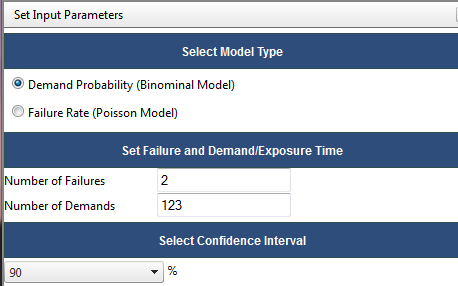
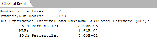
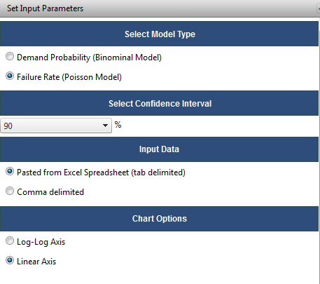
Select the appropriate model type, enter the failures and demands (or time), and select a confidence interval. Based on the above assumptions, the classical calculation results in a maximum likelihood (MLE) estimator and a confidence interval.
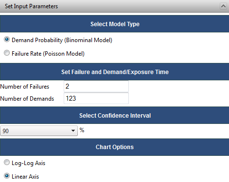
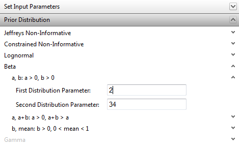
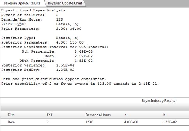
Bayes Update of Un-Partitioned Data
The Bayes menu item allows the user to perform a Bayes estimate. The results of the analysis are based upon the prior distribution of the Jeffreys noninformative distribution, a user-supplied distribution, or a distribution selected from the Distribution bank.
Bayes Estimation of p
Suppose that similar components or systems are repeatedly demanded, and that the following statements are true.
1. The probability of failure on any demand is p, the same for all demands.
2. The success or failure on any demand is independent of the outcomes on other demands.
Under these assumptions, the number of failures in n demands, X, is a random variable with a binomial(n, p) distribution. RADS performs some statistical checks on the plausibility of these assumptions.
Bayesian estimation measures uncertainty in p by a probability distribution. It assumes some prior distribution for p, corresponding to uncertainty in p before taking the present data into account. Five forms of the prior distribution are allowed.
· A beta distribution. The user may specify the distribution by inputting the two standard parameters, or by inputting the mean and one of the standard parameters.
· The Jeffreys noninformative distribution. This is a beta distribution with parameters ½ and ½.
· A (beta approximation of the) constrained noninformative prior distribution. The user must input the mean, and RADS will calculate the dispersion automatically, corresponding in a specific sense to no information other than the mean.
· A lognormal distribution. The user may specify the distribution by inputting the mean and standard deviation of the underlying normal distribution or the mean and error factor of the lognormal distribution, or the median and error factor of the lognormal distribution. RADS prints a warning if the specified distribution causes Pr(p > 1) to be > 0.001.
RADS then checks to see if the data (x failures in n demands) are consistent with the prior distribution. That is, if x/n is less than the prior mean, RADS calculates
![]()
where f is the prior density. If, instead, x/n is greater than the prior mean, RADS calculates
![]()
In either case, if the calculated integral is 0.025 or smaller, RADS prints a warning message that the data and the prior distribution appear to be inconsistent. The user is given the choice of continuing or specifying a new prior distribution.
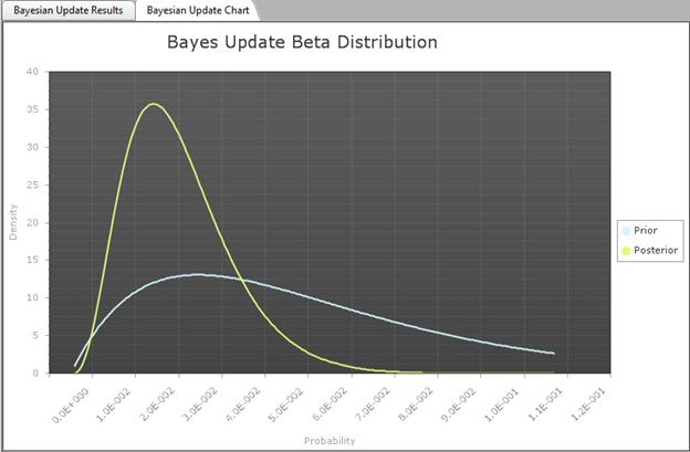
RADS then calculates the posterior distribution, and presents selected percentiles of the distribution, as well as the posterior mean, variance, and standard deviation.
If the prior distribution is a beta distribution, the posterior distribution is also a beta distribution, and all of the calculations are performed algebraically. If the prior distribution is not a beta distribution, all the calculations use numerical integration.
For more information on Bayes estimation of p when using a beta prior, see Atwood (1994) (Ref 3), Box and Tiao (1973) (Ref [1]), or Martz and Waller (1991) (Ref 6).
Bayesian Estimation of Lambda
Suppose that one or more similar components or systems are observed over time, that events, such as failures, occur randomly. Suppose further:
1. The probability of an event in a time interval of length Dt is approximately lDt, with l unchanging.
2. Exactly simultaneous events do not occur.
3. Event occurrences in disjoint time periods are independent.
Under these assumptions, the number of failures in time t is a random variable with a Poisson(lt) distribution. RADS performs some statistical checks on the plausibility of these assumptions.
Bayesian estimation measures uncertainty in l by a probability distribution. It assumes some prior distribution for l, corresponding to uncertainty in l before taking the present data into account. Four forms of the prior distribution are allowed.
1. A gamma distribution. The user may specify the distribution by inputting the two standard parameters, or by inputting the mean and one of the standard parameters.
2. The Jeffreys noninformative distribution. This is an improper distribution (that is, it has an infinite integral), proportional to λ-1/2 . However, in may be treated algebraically as if it were a gamma distribution with parameters 1/2 and 0.
3. A constrained noninformative prior distribution. This is also a gamma distribution. The user must input the mean, and RADS will calculate the dispersion automatically, corresponding in a specific sense to no information other than the mean.
4. A lognormal distribution. The user may specify the distribution by inputting the mean and standard deviation of the underlying normal distribution or the mean and error factor of the lognormal distribution, or the median and error factor of the lognormal distribution.
RADS then checks to see if the data (x events in time t) are consistent with the prior distribution. That is, if x/t is less than the prior mean, RADS calculates
![]() ,
,
where f is the prior density. If, instead, x/n is greater than the prior mean, RADS calculates
![]() .
.
In either case, if the calculated integral is 0.025 or smaller, RADS prints a warning message that the data and the prior distribution appear to be inconsistent. The user is given the choice of continuing or specifying a new prior distribution.
RADS then calculates the posterior distribution, and presents selected percentiles of the distribution, as well as the posterior mean, variance, and standard deviation.
If the prior distribution is a gamma distribution, the posterior distribution is also a gamma distribution, and all of the calculations are performed algebraically. If the prior distribution is not a gamma distribution, all the calculations use numerical integration.
For more information on Bayes estimation of lambda when using a gamma prior, see Engelhardt (1994) (Ref [2]), Box and Tiao (1973) (Ref 1), or Martz and Waller (1991) (Ref 6).
Analysis of Partitioned Data
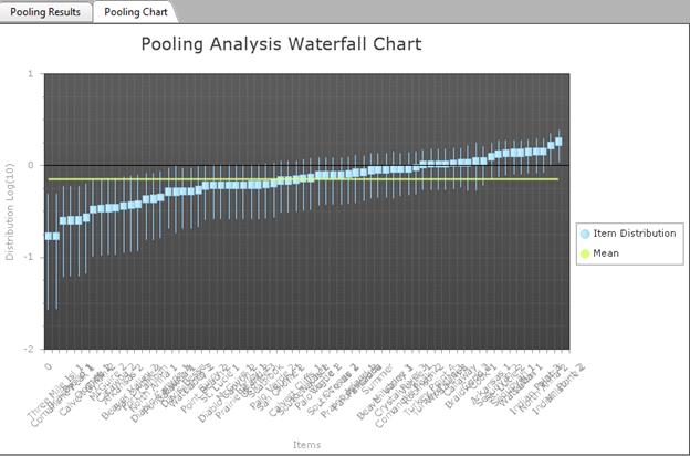
Pooling
Consider random counts that correspond to cells, so that every cell gets some count. For example, the counts could be numbers of failures or successes, and a cell might correspond to failures at a particular plant, or successes of a particular system, or failures during some time period. For more details, see the explanations for testing poolability when estimating p or estimating l. Let ni denote the count for cell i. A hypothesis, Ho is to be tested, such as the hypothesis that all the failures on demand have the same probability or that all the events in time occur with the same frequency. These two example hypotheses each involve an unknown parameter, the failure probability and the event frequency, respectively. In general, the hypothesis to be tested typically involves one or more unknown parameters.
Estimate the unknown parameter(s) from the count data, and
calculate the expected count for each cell if the hypothesis is true. Denote
the expected count for cell i by ![]() . The difference
between the observed count and the expected count for any cell is
. The difference
between the observed count and the expected count for any cell is ![]() . There are many
cells, and therefore many ways of combining the differences to yield an overall
number. One useful way is to construct
. There are many
cells, and therefore many ways of combining the differences to yield an overall
number. One useful way is to construct
![]() ,
,
called the chi-squared statistic, or sometimes the Pearson
chi-squared statistic after its inventor, Karl Pearson. If the observed counts
![]() are far from the expected
values
are far from the expected
values ![]() , the evidence against
Ho is strong. Therefore, Ho should be
rejected if
, the evidence against
Ho is strong. Therefore, Ho should be
rejected if ![]() is large, and not
rejected if
is large, and not
rejected if ![]() is small.
is small.
How large or small must ![]() be? As the counts
become large,
be? As the counts
become large, ![]() has approximately a
chi-squared distribution. To calculate the degrees of freedom, treat any
demand counts as nonrandom. The degrees of freedom is the number of
independent counts, minus the number of estimated parameters under Ho.
Reject Ho if
has approximately a
chi-squared distribution. To calculate the degrees of freedom, treat any
demand counts as nonrandom. The degrees of freedom is the number of
independent counts, minus the number of estimated parameters under Ho.
Reject Ho if ![]() is in the right tail
of the chi-squared distribution, for example beyond the 95th
percentile.
is in the right tail
of the chi-squared distribution, for example beyond the 95th
percentile.
The chi-squared approximation is valid if the data set is
large. RADS gives a mild warning if any of the expected values ![]() are less than 1.0,
and a stronger warning if any of the
are less than 1.0,
and a stronger warning if any of the ![]() values are less than
0.5. These warnings agree with standard published rules of thumb.
values are less than
0.5. These warnings agree with standard published rules of thumb.
This test for poolability does not use any ordering of the cells. Thus, tests that are specifically designed to detect trends may be more suited to analysis of differences between time periods.

Testing for Homogeneity (Poolability) When Estimating p
In the typical RADS application, two attributes of any event
are (a) whether it is a failure or success and (b) the source of the data ¾ the plant, the system, the year, or the
type of demand. RADS constructs a table with two columns and R rows.
The columns correspond to failures and successes, respectively, and the R
rows correspond to the R sources of data. Denote the count in the ith
row and jth column by ![]() , for i any
number from 1 to R and j equal to 1 or 2. The number of failures
for row i is
, for i any
number from 1 to R and j equal to 1 or 2. The number of failures
for row i is ![]() and the number of
successes is
and the number of
successes is ![]() . The number of
demands is
. The number of
demands is ![]() . Similarly, let
. Similarly, let ![]() be the total number
of failures in all rows, let
be the total number
of failures in all rows, let ![]() be the total number
of successes, and let
be the total number
of successes, and let ![]() be the grand total
number of demands.
be the grand total
number of demands.
The hypothesis of poolability is that all the rows
correspond to the same probability of failure on demand. The natural estimate
of this probability is ![]() . If the data sources
can be pooled, the expected number of failures for row i is
. If the data sources
can be pooled, the expected number of failures for row i is ![]() , and the expected
number of successes is
, and the expected
number of successes is ![]() . The Pearson
chi-squared statistic is defined as
. The Pearson
chi-squared statistic is defined as
![]()
If the observed counts are far from the expected counts, the
evidence against poolability is strong. The existence of observed counts that
are far from the expected counts causes ![]() to be large.
Therefore, poolability is rejected when
to be large.
Therefore, poolability is rejected when ![]() is large. When the
sample size is large,
is large. When the
sample size is large, ![]() has approximately a
chi-squared distribution with R -
1 degrees of freedom. So poolability is rejected with p-value 0.05 if
has approximately a
chi-squared distribution with R -
1 degrees of freedom. So poolability is rejected with p-value 0.05 if ![]() is larger than the
95th percentile of the chi-squared distribution, with p-value 0.01 if
is larger than the
95th percentile of the chi-squared distribution, with p-value 0.01 if ![]() is larger than the
99th percentile, and so forth.
is larger than the
99th percentile, and so forth.
The contribution to ![]() from row i is
from row i is
![]() .
.
Inspection of these terms shows which rows show the most deviation from the overall average, in the sense of the chi-squared test. They can help show in what ways poolability is violated. In RADS the signed square root of this term is shown, with a positive sign if the number of failures is higher than expected, and a negative sign if the number of failures is lower than expected. These signed square roots are called the "Pearson residuals."
If the data set is small (few failures or few successes) the
chi-squared approximation is not very good. RADS gives a mild warning if any
of the expected values ![]() are less than 1.0,
and a stronger warning if any of the
are less than 1.0,
and a stronger warning if any of the ![]() values are less than
0.5. These warnings agree with standard published rules of thumb.
values are less than
0.5. These warnings agree with standard published rules of thumb.
For more information, see Atwood (1994) (Ref 3)
Testing for Homogeneity (Poolability) When Estimating Lambda
In the typical RADS application, various sources of the data
¾ plants, systems, years, or types of
discovery activity ¾ each correspond to
a count of events (such as initiating events or system demands) and an exposure
time, such as calendar years or critical hours. RADS constructs a table with C
cells, each cell corresponding to one source of data. The ith
cell contains a count, ni, the number of events reported for
that source of data during exposure time ![]() . Denote the total
number of events in all the data by
. Denote the total
number of events in all the data by ![]() , and denote the total
exposure time by
, and denote the total
exposure time by ![]() .
.
The hypothesis of poolability is that all the cells
correspond to the same event frequency. The natural estimate of this frequency
is ![]() . If the data
sources can be pooled, the expected number of events for cell i is
. If the data
sources can be pooled, the expected number of events for cell i is ![]() . The Pearson
chi-squared statistic is defined as
. The Pearson
chi-squared statistic is defined as
![]() .
.
If the observed counts are far from the expected counts, the
evidence against poolability is strong. The existence of observed counts that
are far from the expected counts causes
![]() to be large.
Therefore, poolability is rejected when
to be large.
Therefore, poolability is rejected when ![]() is large. When the
sample size is large,
is large. When the
sample size is large, ![]() has approximately a
chi-squared distribution with C -
1 degrees of freedom. So poolability is rejected with p-value 0.05 if
has approximately a
chi-squared distribution with C -
1 degrees of freedom. So poolability is rejected with p-value 0.05 if ![]() is larger than the
95th percentile of the chi-squared distribution, with p-value 0.01 if
is larger than the
95th percentile of the chi-squared distribution, with p-value 0.01 if ![]() is larger than the
99th percentile, and so forth.
is larger than the
99th percentile, and so forth.
The contribution to ![]() from row i is
from row i is
![]() .
.
Inspection of these terms shows which cells show the most
deviation from the overall average, in the sense of the chi-squared test. They
can help show in what ways poolability is violated. RADS shows the signed
square root of these terms,![]() . They are called the
"Pearson residuals".
. They are called the
"Pearson residuals".
If the data set is small (few events) the chi-squared
approximation is not very good. RADS gives a mild warning if any of the
expected values ![]() are less than 1.0, and
a stronger warning if any of the
are less than 1.0, and
a stronger warning if any of the ![]() values are less than
0.5. These warnings agree with standard published rules of thumb.
values are less than
0.5. These warnings agree with standard published rules of thumb.
For more information, see Engelhardt (1994) (Ref 2).
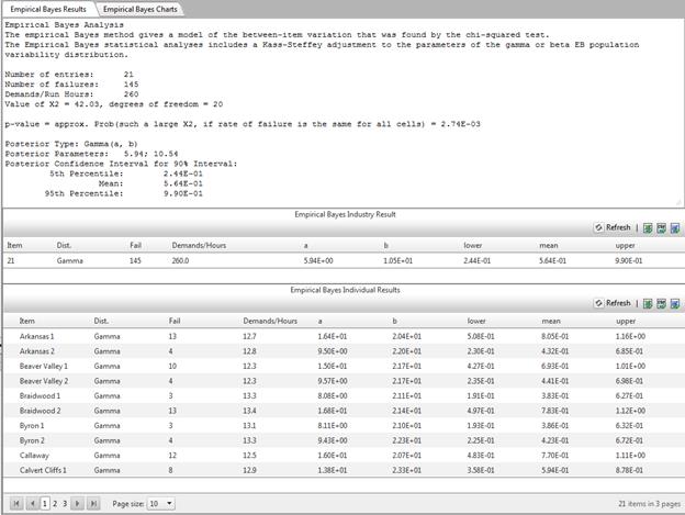
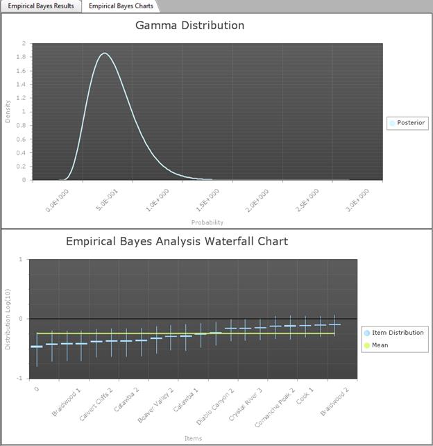
Empirical Bayes
Empirical Bayes estimation is used when the parameter varies. For example, p or Lambda may be different at different plants. It is assumed that the plant-specific parameter is generated randomly from some population-variability distribution. Once the parameter has been generated for a specific plant, data at that plant are randomly produced, with a distribution governed by the plant-specific parameter. This hierarchical model is illustrated for Poisson data in the figure below, with the plant-specific parameters generated at one level and the data for each plant generated at the next level.
Hierarchical model for Poisson data
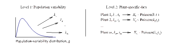
The distribution g involves unknown parameters. If g is a conjugate distribution (a gamma distribution for lambda, or a beta distribution for p), the empiric al Bayes method estimates the two unknown parameters of g from the data, using maximum likelihood estimation.
Empirical Bayes Estimation of p
Suppose that the data for failures on demand have been partitioned into distinct data sources, such as distinct plants or systems. For concreteness, the model is explained here assuming that the distinct data sources are plants. Each plant corresponds to an observed number of demands, say ni demands for the ith plant. The number of failures for that plant is assumed to be a binomial(ni, p) random variable.
Suppose that p is believed to vary from plant to plant. For example, the chi-square test may have rejected the hypothesis of a constant p, or engineering considerations may suggest that p is not constant. What model should be used?
One approach is to analyze each plant separately, resulting in a separate estimate of p for each plant. This is reasonable if there are only two plants. It might also be reasonable if one plant is clearly different from all the others. In this case, the one plant could be analyzed separately, and all the other plants might be considered as a single homogeneous source. After this regrouping of the data, only two data sources exist, to be analyzed separately.
Often, however, removal of one outlier leaves a data set that contains another outlier, and removal of that may leave a set with still another outlier. In such cases it is simpler (that is, it involves fewer parameters to estimate) to use the following compound model.
The method models the variation between the plants, using a population-variability distribution. It is
assumed that p varies from plant to plant, and follows a beta(a, b) distribution. Let ![]() denote the value
corresponding to the ith plant. At this plant,
conditional on the value of
denote the value
corresponding to the ith plant. At this plant,
conditional on the value of ![]() , it is assumed that
each demand results in a failure with probability
, it is assumed that
each demand results in a failure with probability ![]() . In short, the
number of failures in n demands at the ith
plant is binomial(n,
. In short, the
number of failures in n demands at the ith
plant is binomial(n, ![]() ); the number of
failures in n demands at a single random plant has a
beta-binomial(n, a, b) distribution. The value of n
is known, and the two parameters a and b are unknown.
); the number of
failures in n demands at a single random plant has a
beta-binomial(n, a, b) distribution. The value of n
is known, and the two parameters a and b are unknown.
RADS uses numerical iteration to find the maximum likelihood estimates of a and b.
The iterative procedure does not always converge. In some cases, the search for the maximum likelihood leads to a/(a+b) stabilizing at a finite value but a+b diverging to infinity. RADS stops the numerical search whenever a+b appears to be larger than the total number of trials in the data set; such a large value for a+b should not be used because it would result in plant-specific intervals shorter than the interval based on simply pooling all the data. In this case RADS states that the empirical Bayes distribution is degenerate, concentrated at a single point.
Suppose now that finite values of a and b have
been estimated, giving an estimated overall distribution of p. We now
naturally inquire about the value of ![]() at the ith
plant. The model says that
at the ith
plant. The model says that ![]() was randomly selected
from the beta(a, b) distribution, and the
was randomly selected
from the beta(a, b) distribution, and the ![]() failures in ni
demands were generated from a binomial(
failures in ni
demands were generated from a binomial(![]() ,
,![]() ) distribution.
Recall that a and b are estimated. The simplest approach is to
act as if the estimates were the true values. For the ith
data source, let the prior distribution of
) distribution.
Recall that a and b are estimated. The simplest approach is to
act as if the estimates were the true values. For the ith
data source, let the prior distribution of ![]() be beta(a, b),
and find the posterior distribution of
be beta(a, b),
and find the posterior distribution of ![]() by updating the prior
with the data. This is the usual Bayes method for
estimating , except that the
prior parameters are estimated from all the data. This leads to the name
"empirical Bayes estimation."
by updating the prior
with the data. This is the usual Bayes method for
estimating , except that the
prior parameters are estimated from all the data. This leads to the name
"empirical Bayes estimation."
More sophisticated methods account for the variability in the estimators a and b. In particular, Kass and Steffey (1989)(Ref [4]) give a simple first-order correction, which RADS applies to the beta-binomial model. This approach leaves each plant-specific mean unchanged but lengthens the interval somewhat.
RADS gives the overall distribution, beta(a, b), with its mean and a 90% interval corresponding to the 5th and 95 percentiles. RADS also gives the plant-specific means and 90% intervals. The plant-specific distributions are approximated by beta distributions, but after the Kass-Steffey adjustment the plant-specific distribution parameters do not correspond to simple updating of a single prior distribution with the plant-specific data. For more information, see Atwood (1994) (Ref 3) .
Empirical Bayes Estimation of Lambda
Suppose that the data for and event frequency have been
partitioned into distinct data sources, such as distinct plants or systems.
For concreteness, the model is explained here assuming that the distinct data
sources are plants. Each data source corresponds to an observed exposure time,
say ![]() hours for the ith
plant. The number of events for that plant is assumed to be a Poisson(λti)
random variable.
hours for the ith
plant. The number of events for that plant is assumed to be a Poisson(λti)
random variable.
Suppose that l is believed to vary from plant to plant. For example, the chi-square test may have rejected the hypothesis of a constant l, or engineering considerations may suggest that l is not constant. What model should be used?
One approach is to analyze each plant separately, resulting in a separate estimate of l for each plant. This is reasonable if there are only two plants. It might also be reasonable if one plant is clearly different from all the others. In this case, the one plant could be analyzed separately, and all the other plants might be considered as a single homogeneous source. After this regrouping of the data, only two data sources exist, to be analyzed separately.
Often, however, removal of one outlier leaves a data set that contains another outlier, and removal of that may leave a set with still another outlier. In such cases it is simpler (that is, it involves fewer parameters to estimate) to use the following compound model.
The method models the variation between the plants. It is
assumed that l varies from plant
to plant, and follows a gamma (a, b) distribution.
Let ![]() denote the value
corresponding to the ith plant. At this plant, it is
assumed that events occur randomly with frequency
denote the value
corresponding to the ith plant. At this plant, it is
assumed that events occur randomly with frequency ![]() . In short, the
number of failures in time t at the ith plant
is Poisson
. In short, the
number of failures in time t at the ith plant
is Poisson![]() ; the number of
failures in time t demands at a single random plant has a
gamma-Poisson(t, a, b) distribution. The value of t
is known, and the two parameters a and b are unknown.
; the number of
failures in time t demands at a single random plant has a
gamma-Poisson(t, a, b) distribution. The value of t
is known, and the two parameters a and b are unknown.
RADS uses numerical iteration to find the maximum likelihood estimates of a and b.
The iterative procedure does not always converge. In some cases, the search for the maximum likelihood leads to a/b stabilizing at a finite value but b diverging to infinity. RADS stops the numerical search whenever b appears to be larger than the total exposure time in the data set; such a large value for b should not be used because it would result in plant-specific intervals shorter than the interval based on simply pooling all the data. In this case RADS states that the empirical Bayes distribution is degenerate, concentrated at a single point.
Suppose now that finite values of a and b have
been estimated, giving an estimated overall distribution of l. We now naturally inquire about the
value of ![]() at the ith
plant. The model says that
at the ith
plant. The model says that ![]() was randomly selected
from the gamma(a, b) distribution, and the
was randomly selected
from the gamma(a, b) distribution, and the ![]() events in time
events in time ![]() were generated from a
Poisson
were generated from a
Poisson![]() distribution. Recall
that a and b are estimated. The simplest approach is to act as
if the estimates were the true values. For the ith
data source, let the prior distribution of
distribution. Recall
that a and b are estimated. The simplest approach is to act as
if the estimates were the true values. For the ith
data source, let the prior distribution of ![]() be beta(a, b),
and find the posterior distribution of
be beta(a, b),
and find the posterior distribution of ![]() by updating the prior
with the data. This is the usual Bayes method for
estimating
by updating the prior
with the data. This is the usual Bayes method for
estimating ![]() , except that the
prior parameters are estimated from all the data. This leads to the name
"empirical Bayes estimation."
, except that the
prior parameters are estimated from all the data. This leads to the name
"empirical Bayes estimation."
More sophisticated methods account for the variability in the estimators a and b. In particular, Kass and Steffey (1989) (Ref 5) give a simple first-order correction, which RADS applies to the gamma-Poisson model. This approach leaves each plant-specific mean unchanged but lengthens the interval somewhat.
RADS gives the overall distribution, gamma(a, b), with its mean and a 90% interval corresponding to the 5th and 95 percentiles. RADS also gives the plant-specific means and 90% intervals. The plant-specific distributions are approximated by gamma distributions, but after the Kass-Steffey adjustment the plant-specific distribution parameters do not correspond to simple updating of a single prior distribution with the plant-specific data. For more information, see Engelhardt (1994) (Ref 3).
Trending
Estimating a Trend in p
Model of trend
The model is the same as when estimating a failure probability (see also Bayesian Estimation of p), except now the probability p depends on time, t. Thus, the model assumptions are
1. A demand at time t results in a failure with some probability p(t), and a success with probability 1 - p(t).
2. Occurrences of failures on different demands are statistically independent.
By far the most commonly used functional form for p(t) is the logit model, in which ln{ p(t)/[1 - p(t)] } is a simple function of unknown parameters. Fitting such a model to data is sometimes called logistic regression. RADS uses this model, and fits
ln{ p(t)/[1 - p(t)] } = a + bt .
This function of p has a name, the logit function. Therefore, the above equation could be written
logit[p(t)] = a + bt .
A frequently used relation is that
y = logit[p(t)] / ln{ p(t)/[1 ! p(t)] }
is equivalent to
p(t) = logit![]() (y) /
(y) / ![]() ,
,
denoting the inverse function of the logit by logit-1. The figure below shows p(t) as a function of t, where logit[p(t)] = a + bt, with a = 0.1 and several values of b. Notice that the value of p(t) stays between 0.0 and 1.0, as it should.
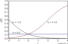
The parameters have simple interpretations: a is the value of the logit of p when t = 0, and b is the slope of the logit of p.
The model assumes that logit[p(t)] = a + bt . Therefore, one might decide simply to use least-squares software as follows. First, estimate p for each bin, based on only the data for that bin:
![]() .
.
Then fit logit![]() to
to ![]() by least squares.
The same problems must be addressed that are mentioned for fitting a rate l.
by least squares.
The same problems must be addressed that are mentioned for fitting a rate l.
First, if any observed failure count, ![]() , equals either 0 or
the demand count ni, then
, equals either 0 or
the demand count ni, then ![]() will be 0.0 or 1.0
for that bin, and the logit will be undefined. RADS offers three choices.
will be 0.0 or 1.0
for that bin, and the logit will be undefined. RADS offers three choices.
1.
Estimate
![]() by
by ![]() , the MLE. This method fails if
, the MLE. This method fails if
![]() = 0 or
= 0 or ![]() = ni for any bin, because
then logit
= ni for any bin, because
then logit![]() is undefined.
is undefined.
2.
Instead
of estimating ![]() by
by ![]() , use
, use ![]() . This is equivalent
to replacing the MLE by the posterior mean based on the Jeffreys noninformative prior.
. This is equivalent
to replacing the MLE by the posterior mean based on the Jeffreys noninformative prior.
3.
Estimate
![]() by the posterior mean
based on the constrained noninformative prior. In this case, the constraint is that
the prior mean equals
by the posterior mean
based on the constrained noninformative prior. In this case, the constraint is that
the prior mean equals ![]() . This is the default
method.
. This is the default
method.
Such ways tend to reduce the trend slightly, because they add a constant to all the failure and demand counts, slightly flattening out any original differences. Using a constrained noninformative prior has a smaller such effect than using the Jeffreys prior.
The second point that must be considered is that the
variance of the estimator of p is not constant. Therefore, the
following iteratively reweighted least-squares method can be used. Assume that
p in the ith bin is estimated by ![]() . If the simple MLE
is used, then a and b are both zero. If method 1 above is
used, then a = 2 and b = 2.
If method 2 above is used, then a
and b must be found from a table
for the constrained noninformative prior. Neter and Wasserman (1974, Eq.
(9.51)) (Ref 5) state that the asymptotic variance of logit[MLE of
. If the simple MLE
is used, then a and b are both zero. If method 1 above is
used, then a = 2 and b = 2.
If method 2 above is used, then a
and b must be found from a table
for the constrained noninformative prior. Neter and Wasserman (1974, Eq.
(9.51)) (Ref 5) state that the asymptotic variance of logit[MLE of ![]() ] is
] is
![]()
The method given here is a generalization when a and b
are not both zero, setting the weight ![]() to the inverse of the
asymptotic variance of the estimator.
to the inverse of the
asymptotic variance of the estimator.
Begin by assuming that p is constant, and let ![]() be some simple
estimate of p, the same for all i. Fit
be some simple
estimate of p, the same for all i. Fit
![]()
to a straight line with weighted least squares, and weights
![]() .
.
Calculate the resulting estimates of ![]() ,
,
![]() .
.
Recalculate the weights with these estimates, and refit the data to a straight line using weighted least squares. Repeat this process until the estimates stabilize.
The final point is that least-squares fitting typically
assumes that the data are approximately normally distributed around the
straight line. In the present context, this means that logit(![]() ) is assumed to be
approximately normally distributed. This assumption is acceptable, unless the
total number of failures is close to zero or to the total number of demands.
However, the variance of the normal distribution is then estimated from the
scatter around the fitted line. This differs from typical treatment of
binomial data, where the mean determines the variance.
) is assumed to be
approximately normally distributed. This assumption is acceptable, unless the
total number of failures is close to zero or to the total number of demands.
However, the variance of the normal distribution is then estimated from the
scatter around the fitted line. This differs from typical treatment of
binomial data, where the mean determines the variance.
A 90% confidence interval for p(t) at a particular t is given by
![]() (1)
(1)
Where ![]() is the 95th percentile
of Students t distribution with df degrees of freedom.
is the 95th percentile
of Students t distribution with df degrees of freedom.
The above confidence interval
is for a particular t. For many values of t, many such confidence
intervals could be calculated. Each is a valid confidence interval, but they
are not simultaneously valid. This is a subtle point. To appreciate it,
recall the interpretation of the 90% confidence
interval for l(t) for
some particular time ![]() :
:
Pr[confidence interval for p(![]() contains true
occurrence rate at time
contains true
occurrence rate at time ![]() ] = 0.90. (2)
] = 0.90. (2)
Here, the data set is thought of as random. If many data
sets could be generated from the same set of years, each data set would allow
the calculation of a confidence interval for ![]() , and 90% of these
confidence intervals would contain the true occurrence rate.
, and 90% of these
confidence intervals would contain the true occurrence rate.
A similar confidence statement applies to each time. The simultaneous statement would involve
Pr[confidence
interval for p(![]() contains true
occurrence rate at time
contains true
occurrence rate at time ![]() AND
AND
confidence
interval for p(![]() contains true
occurrence rate at time
contains true
occurrence rate at time ![]() AND
AND
so forth ]. (3)
This probability is hard to quantify, because the intervals are all calculated from the same data set, and thus are correlated. However, Expression (3) is certainly smaller than 0.90, because the event in square brackets in Expression (3) is more restrictive that the event in brackets in Eq. (2).
This problem is familiar in the context of least squares
fitting. For example, Neter and Wasserman (1974) (Ref 5) discuss it, and attribute the solution to Working, Hotelling, and Scheffé. A simultaneous 90%
confidence band has the same form as (1), but the multiplier ![]() is replaced by
is replaced by
![]() ,
,
Where ![]() is the 90th
percentile of the F distribution with 2 and df degrees of
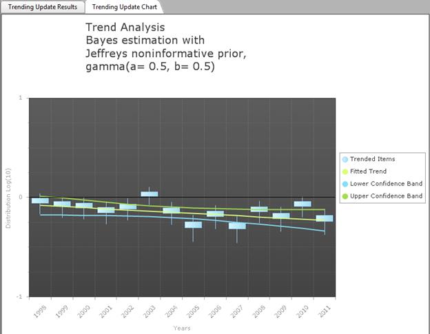
freedom. RADS gives a plot of the fitted trend and of the simultaneous
confidence band for the trend line.
is the 90th
percentile of the F distribution with 2 and df degrees of
freedom. RADS gives a plot of the fitted trend and of the simultaneous
confidence band for the trend line.
For better or worse, this method does not use the assumption that the counts in each bin are binomially distributed. It instead uses the assumption that the estimated frequency for each bin is approximately logistic-normally distributed.
Test for presence of trend
Let the two hypotheses be defined by
Ho: p(t) is constant
![]()
The null hypothesis Ho is false if and only if b is nonzero. Therefore, the test of Ho is the same as a test that b = 0. This test is carried out, based on the estimate of b and the standard error of the estimate, and the assumption that the points being fitted have approximately normal scatter around the trend line. RADS reports the result of this test.
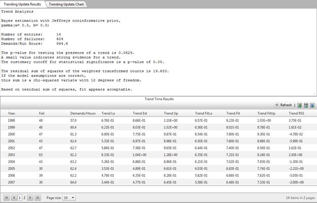
Model Validation
RADS constructs a weighted sum of squares that should have approximately a chi-squared distribution if the model assumptions are valid. A very large value is evidence that the model does not fit the data well. RADS calculates the p-value for lack of fit, the probability that the sum of squares would be as large as observed or larger, if the model assumptions are valid.
In addition, RADS reports a "standardized residual" for each bin. (The above sum of squares equals the sum of the squared standardized residuals.) Examination of the standardized residuals can help show which bins, if any, are contributing most heavily to lack of fit.
If the weighted sum of squares is in the right tail of the chi-squared distribution, such as beyond the 95th percentile, this is evidence of lack of fit. One common causes of lack of fit is systematic variation C the assumed form of the model is incorrect. That means that logit[p(t)] is not of the form a + bt. Another possible cause is extra-Poisson variance, additional sources of variation that are not accounted for in the Poisson model. To gain insight as to which contributors to lack of fit seem to be present, examine the standardized residuals, and the plot given by RADS. Look to see if the variation appears to be systematic or random.
Estimating a Trend in Lambda
Model of trend
This model is the same as when estimating an event frequency lambda (see Frequentist Estimation of Lambda, and Bayesian Estimation of Lambda), except now the frequency l depends on time t. The setting is that one or more similar components or systems are observed over time, and that events, such as failures occur randomly. Suppose the following.
1. The probability of an event in a time interval of length Dt approaches 0 as Dt ® 0. This assumption says that the probability of an event occurring in any short interval (t, t + Dt) is approximately l(t)Dt for some function of t, l(t).
2. Exactly simultaneous events do not occur.
3. Event occurrences in disjoint time periods are independent.
The assumed model is an extension of the model for a homogeneous Poisson process.
RADS considers two important special cases.
1. l(t) = a constant > 0. In this case, the constant is denoted l.
2. l(t) = exp(a + bt), where t measures time and a and b are unknown parameters, which must be estimated from the data. This is called a loglinear model, because lnl(t) = a + bt. It is also called the exponential event rate model. Here, b has units 1/time.
In the second case, l(t) is increasing if b is positive and decreasing if b is negative. If b equals 0, the model reduces to the first case, with constant l. Tests for trend are formulated as tests of whether b = 0. Note also that the occurrence rate is positive in both cases.
The interpretation of a is the intercept of lnl(t), that is, the value of l(t) at t = 0. The meaning of a depends on how time is coded. The time period for the data is divided into bins. Typically, RADS codes time so that the first data bin corresponds to t = 1.
Estimation
The bins must be small enough that l(t) is approximately a
straight-line function within each bin, not strongly curved within the bin.
Denote the midpoint of the ith bin by ![]() . Then the expected
number of events in the bin is approximately
. Then the expected
number of events in the bin is approximately ![]() , where
, where ![]() is the exposure time for the bin. The method is to fit
the observed counts
is the exposure time for the bin. The method is to fit
the observed counts![]() , to
, to ![]() , while assuming that
, while assuming that ![]() has some parametric
form.
has some parametric
form.
Since the model assumes
ln(l(t)) = a + bt
it would seem simple to use least-squares software as follows. First, estimate l in each bin based only on the data for that bin:
![]()
Then fit ln![]() to
to ![]() by least squares. In
principle, this works. In practice, the method has several twists in the road,
described next.
by least squares. In
principle, this works. In practice, the method has several twists in the road,
described next.
First, if the observed count is zero in any bin, ![]() will be zero for that
bin, and the logarithm will be undefined. RADS offers the user three choices
will be zero for that
bin, and the logarithm will be undefined. RADS offers the user three choices
1.
Estimate
![]() by
by ![]() , the MLE. This method fails if
any
, the MLE. This method fails if
any ![]() is zero, because ln(0)
is undefined.
is zero, because ln(0)
is undefined.
2.
Estimate
![]() by
by ![]() . This is equivalent
to replacing the MLE by the posterior mean based on the Jeffreys noninformative prior.
. This is equivalent
to replacing the MLE by the posterior mean based on the Jeffreys noninformative prior.
· Estimate ![]() by the posterior mean
based on the constrained noninformative prior.
In this case, the constraint is that the prior mean equals
by the posterior mean
based on the constrained noninformative prior.
In this case, the constraint is that the prior mean equals ![]() . This is the default
method.
. This is the default
method.
Such ways tend to reduce the trend slightly, because they add a constant to all the event counts, slightly flattening out any original differences. Using a constrained noninformative prior has a smaller such effect than using the Jeffreys prior.
The second point that must be considered is that the
variance of ![]() is not constant. For
simplicity, this issue will be explained for the case with no zero counts, and
ln(
is not constant. For
simplicity, this issue will be explained for the case with no zero counts, and
ln(![]() estimated by ln
estimated by ln![]() = ln(
= ln(![]() ).
).
The variance of ln(![]() ) is approximately the
relative variance of
) is approximately the
relative variance of ![]() , which is
, which is
![]()
If ![]() has a Poisson
has a Poisson![]() distribution.
Ordinary least-squares fitting has some optimality properties if the variance
is constant. Otherwise, it is more efficient to use weighted least squares,
with weights inversely proportional to the variances of the observations.
distribution.
Ordinary least-squares fitting has some optimality properties if the variance
is constant. Otherwise, it is more efficient to use weighted least squares,
with weights inversely proportional to the variances of the observations.
Unfortunately, the variances depend on the ![]() values, which are
unknown. Therefore, the following iteratively reweighted least-squares
method is used. Begin by assuming that l
is constant, and fit ln(
values, which are
unknown. Therefore, the following iteratively reweighted least-squares
method is used. Begin by assuming that l
is constant, and fit ln(![]() ) to a straight line
with weighted least squares, and weights
) to a straight line
with weighted least squares, and weights ![]() . Calculate the
resulting estimates of
. Calculate the
resulting estimates of ![]() ,
,
![]() .
.
Then refit the data to a straight line, using weighted
least squares, and weights ![]() . Repeat this process
until the estimates stabilize.
. Repeat this process
until the estimates stabilize.
The final point is that least-squares fitting typically
assumes that the data are approximately normally
distributed around the straight line. In the present context, this
means that ln(![]() ) is assumed to be
approximately normally distributed. This assumption is acceptable, unless the
mean count is close to zero. However, the variance of the normal distribution
is then estimated from the scatter around the fitted line. This differs from
the typical treatment of Poisson data, where the mean determines the variance.
) is assumed to be
approximately normally distributed. This assumption is acceptable, unless the
mean count is close to zero. However, the variance of the normal distribution
is then estimated from the scatter around the fitted line. This differs from
the typical treatment of Poisson data, where the mean determines the variance.
A 90% confidence interval for l(t) at a particular t is given by
![]() . (1)
. (1)
Here ![]() is the 95th percentile
of Student=s
t distribution with df degrees of freedom.
is the 95th percentile
of Student=s
t distribution with df degrees of freedom.
The above confidence interval
is for a particular time t. For many values of t, many such
confidence intervals could be calculated. Each is a valid confidence interval,
but they are not simultaneously valid. This is a subtle point. To appreciate
it, recall the interpretation of the 90% confidence interval for ![]() for some particular
time
for some particular
time ![]() :
:
Pr[confidence
interval for ![]() contains true
occurrence rate at time
contains true
occurrence rate at time ![]() ] = 0.90. (2)
] = 0.90. (2)
Here, the data set is thought of as random. If many data
sets could be generated from the same set of years, each data set would allow
the calculation of a confidence interval for ![]() , and 90% of these confidence intervals would contain the true
occurrence rate.
, and 90% of these confidence intervals would contain the true
occurrence rate.
A similar confidence statement applies to each time. The simultaneous statement would involve
Pr[confidence
interval for ![]() contains true
occurrence rate at time
contains true
occurrence rate at time ![]() AND
AND
confidence
interval for ![]() contains true
occurrence rate at time
contains true
occurrence rate at time ![]() AND
AND
so forth ]. (3)
This probability is hard to quantify, because the intervals are all calculated from the same data set, and thus are correlated. However, Expression (3) is certainly smaller than 0.90, because the event in square brackets in Expression (3) is more restrictive that the event in brackets in Eq. (2).
This problem is familiar in the context of least squares
fitting. For example, Neter and Wasserman (1974)
(Ref [5]) discuss it, and attribute the
solution to Working, Hotelling, and Scheffé. A simultaneous 90% confidence
band has the same form as (1), but the multiplier ![]() is replaced by
is replaced by
![]() ,
,
where ![]() is the 90th percentile
of the F distribution with 2 and df
degrees of freedom. RADS gives a plot of the fitted trend and of the
simultaneous confidence band for the trend line.
is the 90th percentile
of the F distribution with 2 and df
degrees of freedom. RADS gives a plot of the fitted trend and of the
simultaneous confidence band for the trend line.
For better or worse, this method does not use the assumption that the counts in each bin are Poisson distributed. It instead treats the estimated frequency for each bin as approximately lognormally distributed.
Test for presence of trend
Let the two hypotheses be defined by
Ho: l(t) is constant
H1: l(t) = exp(a + bt), b ¹ 0
The null hypothesis Ho is false if and only if b is nonzero. Therefore, the test of Ho is the same as a test that b = 0. This test is carried out, based on the estimate of b and the standard error of the estimate, and the assumption that the points being fitted have approximately normal scatter around the trend line. RADS reports the result of this test.
Model Validation
RADS constructs a weighted sum of squares that should have approximately a chi-squared distribution if the model assumptions are valid. A very large value is evidence that the model does not fit the data well. RADS calculates the p-value for lack of fit, the probability that the sum of squares would be as large as observed or larger, if the model assumptions are valid.
In addition, RADS reports a "standardized residual " for each bin. (The above sum of squares equals the sum of the squared standardized residuals.) Examination of the standardized residuals can help show which bins, if any, are contributing most heavily to lack of fit.
If the weighted sum of squares is in the right tail of the chi-squared distribution, such as beyond the 95th percentile, this is evidence of lack of fit. One common causes of lack of fit is systematic variation ¾ the assumed form of the model is incorrect. That means that lnl(t) is not of the form a + bt. Another possible cause is extra-Poisson variance, additional sources of variation that are not accounted for in the Poisson model. To gain insight as to which contributors to lack of fit seem to be present, examine the standardized residuals, and the plot given by RADS. Look to see if the variation appears systematic or random.
Curve Fitting
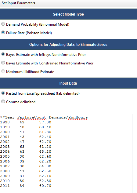
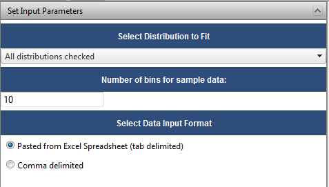
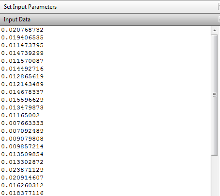
The RADS Calculator implements a limited curve fitting capability for data samples (in a single column of data to be fit). Enter the data manually with a return after each entry or copy and paste from Excel (tab delimited).
Select which distributions to fit the data to (‘All Distributions’ is the default).
The number of bins for the sample data only affects the plotting of the data and defaults to 10.
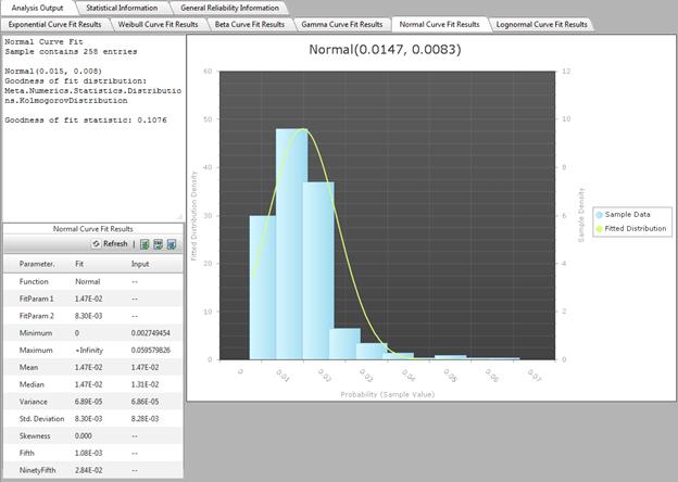
Once the curve fit has been executed, the curve fit results tabs that succeeded (sometimes the curve fitting routine cannot fit the data to the specified curve) will be enabled. The text box provides the parameters of the fitted distribution and a Goodness of Fit Statistic. The larger the Goodness of Fit Statistic, the better the fit.
The grid shows the full range of fitted distribution parameters and the input parameters. The plot shows the binned sample data and the fitted distribution.
The curve fitting routines are provided by a mathematical package named Meta.Numerics. The results have been validated using @Risk and are comparable to those results.
Distributions
Beta distribution
The beta distribution is most commonly used as a Bayes distribution to model uncertainty in a parameter p. The density is
![]() for 0 < p<
1
for 0 < p<
1
For most applications the gamma functions in the front can be ignored ¾ they only form a normalizing constant, to ensure that the density integrates to 1. The important feature of the density is that
![]() ,
,
where the symbol µ denotes “is proportional to.” The parameters of the distribution, a and b, must both be positive. The shape of the beta density depends on the size of the two parameters. If a < 1, the exponent of p is negative in equation for the density, and therefore the density is unbounded as p ® 0. Likewise, if b < 1, the density is unbounded as p ® 1. If both a > 1 and b > 1, the density is roughly bell shaped, with a single mode.
The mean and variance of the distribution are:
mean, denoted m here, = a/(a + b)
variance = m(1 - m)/(a + b + 1).
The formula for the variance shows that as the sum a + b becomes large, the variance becomes small, and the distribution becomes more tightly concentrated around the mean. Although the moments are algebraic functions of the parameters, the percentiles are not so easily found. RADS finds the percentiles of a beta distribution using rather elaborate numerical calculations.
Two beta distributions are plotted below.
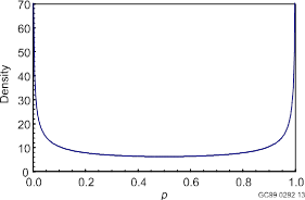
Beta(0.5, 0.5) density. This is the Jeffreys noninformative prior distribution for p.
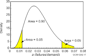
Beta(5.2, 160.1) density, with 5th and 95th percentiles shown. The mean is 5.2/(5.2+160.1) = 0.0315, and the standard deviation is [0.0315(1 - 0.0315)/(5.2 + 160.1 + 1)]1/2 = 0.0135.
The beta distributions form the conjugate family for binomial data. That is, suppose that independent failures and successes are observed, with Pr(failure) = p on each demand. Denote the total number of failures by x and the total number of demands by n. If the prior distribution for p is a beta distribution with parameters aprior and bprior , then the posterior distribution is also a beta distribution, with
aposterior = aprior + x
bposterior = bprior + (n - x) .
This gives an intuitive interpretation for the prior parameters: aprior is to the effective number of failures in the prior information, and bprior is the effective number of successes in the prior information.
RADS allows a beta distribution to be specified by entering any two of: a, b, and m. RADS then calculates and displays the third value.
Gamma distribution
The gamma distribution has many uses. An important use in RADS is as a Bayes prior distribution for a frequency l. For this application, the most convenient parameterization is
![]() for l > 0 .
for l > 0 .
For most applications the terms that do not involve l can be ignored ¾ they only form a normalizing constant, to ensure that the density integrates to 1. The important feature of the density is that
![]()
where the symbol µ denotes “is proportional to.” The parameters of the distribution, a and b, must both be positive.
Some references use other letters for the parameters a and b, and in some applications it is more convenient to parameterize in terms of b¢ = 1/b. The two parameters must both be positive. Here l has units 1/time and q has units of time, so the product lq is unitless. For example, if l is the frequency of events per critical-year, q has units of critical-years. The parameter q corresponds to the scale of l C if we convert l from 1/hours to 1/years by multiplying it by 8760, we correspondingly divide q by 8760, converting it from hours to years. The other parameter, a, is unitless, and is called the shape parameter. The gamma function, G(a), is a standard mathematical function; if a is a positive integer, G(a) equals (a!1)!
The shape of the gamma density depends on the first parameter. If a < 1, the exponent of l is negative in the equation for the density, and therefore the density is unbounded as l ® 0. If a > 1, the density is roughly bell shaped (though skewed to the right), with a single mode. As a ® ¥, the density becomes symmetrical around the mean.
The mean and variance of the distribution are:
mean = a/q
variance = a/q2.
Note that the units are correct, units 1/time for the mean and 1/time2 for the variance. The percentiles of the gamma distribution are calculated by RADS using numerical algorithms. A typical gamma density is plotted below.
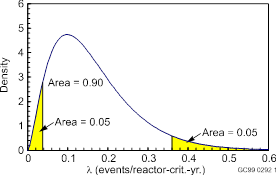
Gamma density with a = 2.53 and b = 15.52 reactor-critical-years. The 5th and 95th percentiles are also shown.
The gamma distributions form a conjugate family for Poisson data. That is, suppose that events occur independently of each other in time, with Pr(an event occurs in time interval of length Dt) » lDt. Let x be the number of events observed in a time period of length t. If l has a gamma prior distribution with parameters aprior and bprior, then the posterior distribution is also a gamma distribution, with
aposterior = aprior + x
bposterior = bprior + t .
This gives an intuitive interpretation for the prior parameters: aprior is to the effective number of events in the prior information, and bprior is the corresponding effective time period in the prior information.
One “distribution” that is often used is the Jeffreys noninformative prior, defined for events in time as a gamma(0.5, 0) distribution. In fact, this is not a distribution, because the second parameter is not positive. Ignoring that problem and taking the limit of a gamma(a, b) density as b ® 0, the density is seen to be proportional to
![]() .
.
This function does not have a finite integral. Therefore, it is not a density, and cannot be made into a density by multiplication by some suitable normalizing constant. It is called an “improper distribution.” Nevertheless, it may be treated as a density in formal algebraic calculations given above, yielding
aposterior = aprior + x = x + 0.5
bposterior = bprior + t = t + 0 = t .
The Jeffreys noninformative prior distribution is plotted below.
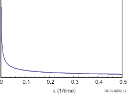
Jeffreys noninformative prior distribution for l, defined as l-1/2 .
RADS allows a gamma distribution to be specified by the α parameter, which is also known as r.
Normal distribution
The normal distribution is not used directly by RADS, but it is used indirectly, in calculations with the lognormal or logistic-normal distributions.
X is normally distributed with mean m and variance s2 if its density is of the form
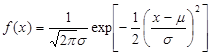 .
.
The parameter m can have any value, and the parameter s must be positive. This density is positive for all x, positive and negative. That is, a normally distributed random variable can take any value, positive or negative.
The mean of the distribution is m and the variance is s2. Percentiles or probabilities involving X can be found from a table of the standard normal distribution, that is, the normal distribution with mean 0 and variance 1. This is done using the following fact. If X has a normal(m, s2) distribution, then (X - m)/s has a normal(0, 1) distribution. For example, suppose that X is normal with m = -3.4 and m and s = 1.2, and the 95th percentile of X is needed. This is the number a such that Pr(X £ a) = 0.95. The desired number is found by solving
0.95 = Pr(X £ a)
Pr[(X - m)/s £ (a - m)/s ] performing the same algebra on both sides of the inequality
Pr[Z £ (a - m)/s] denoting (X - m)/s by Z, where Z is normal(0, 1)
Therefore, (a - m)/s must equal 1.645, because a table of the standard normal distribution shows that 1.645 is the 95th percentile of the distribution. Algebraic rearrangement then shows that
a = m + 1.645s .
Lognormal distribution
Y has a lognormal distribution if ln(Y) has a normal distribution. For use in formulas, denote ln(Y) by X here. Then Y = exp(X). X can take all real values, implying that Y can take all positive values. In Bayesian estimation, an event frequency, l, is sometimes given a lognormal prior distribution. A probability of failure, p, is also sometimes assigned a lognormal prior distribution, even though a lognormal variable can take all possible positive values and p must be £ 1. This conflict is of negligible importance if the lognormal distribution assigns almost all the probability to the interval from 0 to 1.
Let Y be lognormally distributed. That is X = ln(Y) has a normal(m, s2) distribution. The density of Y satisfies
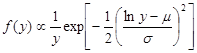 .
.
It is important to note that this is not simply the normal density with lny substituted for x. A 1/y term is also present that does not correspond to anything in the normal density. [The 1/y term enters when (1/y)dy is used to replace dx, similar to the change-of-variables rule in calculus.]
The mean and variance of Y are
mean = exp(m + s2/2)
variance = exp(2m + s2)[exp(s2) - 1] .
The percentiles are obtained by direct translation from the normal distribution: qth percentile of Y = exp(qth percentile of X). In particular
median = exp(m)
95th percentile = exp(m + 1.645s)
5th percentile = exp(m - 1.645s) .
It follows that the error factor, defined as the ratio of the 95th percentile to the median, is
EF = exp(1.645s) .
RADS allows a lognormal distribution to be specified in several ways, according to which pair of inputs the user chooses to enter: either m and s, or the mean and error factor, or the median and error factor. Any of these pairs uniquely determines the distribution. RADS then calculates and displays the other values.
Logistic-normal distribution
The distribution of p has a logistic-normal distribution if ln[p/(1 - p)] has a normal distribution. The function ln[p/(1 - p)] is called the logit function of p. For use in formulas, denote ln[p/(1 - p)] by X here. Then p = exp(X)[1 + exp(X)]. X can take all real values, implying that p can take all values between 0 and 1. This makes the logistic-normal a natural prior distribution for a probability p, although it has not been widely used in PRA applications. If p is small with high probability, the term (1 - p) is usually close to 1, and logit(p) is usually close to ln(p). Therefore, the logistic-normal and lognormal distributions are nearly the same, unless p can take relatively large values (say 0.1 or larger) with noticeable probability.
The moments of the logistic-normal distribution apparently are not given by simple formulas. The percentiles, on the other hand, are obtained by direct translation from the normal distribution: qth percentile of p = exp(qth percentile of X)/{1 + exp(qth percentile of X)]. In particular
median = exp(m)/[1 + exp(m)]
95th percentile = exp(m + 1.645s)/[1 + exp(m + 1.645s)]
RADS allows a logistic-normal distribution to be specified in two ways, according to which pair of inputs the user chooses to enter: either m and s, or the median and 95th percentile. Either of these pairs uniquely determines the distribution. RADS then calculates and displays the other values.
Binomial distribution
The standard model for failures on demand assumes that the number of failures has a binomial distribution. The following assumptions lead to this distribution.
1. Each demand is a failure with some probability p, and is a success with probability 1 ! p.
2. Occurrences of failures for different demands are statistically independent; that is, the probability of a failure on one demand is not affected by what happens on other demands.
Under these assumptions, the number of failures, X, in some fixed number of demands, n, has a binomial(n, p) distribution,
![]()
where
![]() .
.
This distribution has two parameters, n and p, of which only the second is treated as unknown by RADS. The mean of the binomial(n, p) distribution is np, and the variance is np(1 - p).
Assumption 1 says that the probability of failure on demand is the same for every demand. If data are collected over a long time period, the assumption requires that the failure probability does not change or (less realistically) that the analyst does not care if it changes because only the average probability of failure on a random demand is needed. Likewise, if the data are collected from various plants, the assumption is that p is the same at all plants, or that the analyst does not care about between-plant differences but only about the industry average.
Assumption 2 says that the outcome of one demand does not influence the outcomes of later demands. Presumably, events at one plant have little effect on events at a different plant. However, the experience of one failure might cause a change in procedures or design that reduces the failure probability on later demands at the same plant. The binomial distribution assumes that such effects are negligible.
RADS tries to check the data for violations of the assumptions. Thus, it looks for differences between plants or over time. If variation is seen between plants or between systems, RADS allows for a more general model, the empirical Bayes model. If variation is seen over time, RADS allows for modeling of a trend in p.
Poisson distribution
The standard model for events in time assumes that the event count has a Poisson distribution. The following assumptions lead to this distribution.
1. The probability that an event will occur in any specified short exposure time period is approximately proportional to the length of the time period. In other words, for an interval of length Dt the probability of an occurrence in the interval is approximately l H Dt for some l > 0.
2. Exactly simultaneous events do not occur.
3. Occurrences of events in disjoint exposure time periods are statistically independent.
Under the above assumptions, the number of occurrences X in some fixed exposure time t is a Poisson distributed random variable with mean m = lt,
![]() for x = 0,
1, 2, …
for x = 0,
1, 2, …
The parameter l is a rate or frequency. To make things clearer, the kind of event is often stated, that is, “initiating event rate” or “very-small-LOCA frequency.” Because the count of events during a fixed period is a unitless quantity, the mean number of occurrences m is also unitless. However, the rate l depends on the units for measuring time. In other words, the units of l are 1 per unit of time, such as 1/reactor-year or 1/component-hr.
This model is called a Poisson process. It is extremely simple, because it is completely specified by the exposure time, t, and the one unknown parameter, l. Assumption 1 implies that the rate l does not change, neither with a monotonic trend, nor cyclically, nor in any other way. Assumption 2 says that exactly simultaneous events do not occur. The only way that they could occur (other than by incredible coincidence) is if some synchronizing mechanism exists, a common cause. Therefore, the operational interpretation of Assumption 2 is that common-cause events do not occur. Assumption 3 says that the past history does not affect the present. In particular, occurrence of an event yesterday does not make the probability of another event tomorrow either more or less likely. This says that the events do not tend to occur too much in clusters, nor do they tend to be systematically spaced and evenly separated.
RADS tries to check the data for violations of the assumptions. Thus, it looks for differences between plants or over time. If variation is seen between plants or between systems, RADS allows for a more general model, the empirical Bayes model. If variation is seen over time, RADS allows for modeling of a trend in l.
The mean and variance of a Poisson(m) distribution are both equal to m.
Chi-squared Distribution
The chi-squared distribution has many applications in statistics, and therefore is tabulated in most statistics books. In RADS it is used as an approximate distribution of the Pearson chi-squared statistic, valid for large sample sizes. It can also be used to calculate confidence intervals for event frequencies. The density depends on a single positive parameter, called the degrees of freedom. Several chi-squared densities are illustrated here, for different degrees of freedom.
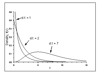
Chi-squared densities with 1, 2, and 7 degrees of freedom.
The formula for a chi-squared density with n degrees of freedom is
, for x ³ 0.
The chi-squared distribution is a special case of a gamma distribution. Indeed, a table of the chi-squared distribution can be used to find probabilities for quantities having gamma distributions.
F Distribution
The F distribution can be used to find a confidence interval for a probability p. Mathematically, the F distribution can be developed as the distribution of the ratio of two random variables with chi-squared distributions. Therefore, the F distribution has two parameters, called the numerator (or first) degrees of freedom and the denominator (or second) degrees of freedom.
Many statistics books tabulate a few upper percentiles of the F distribution, such as the 95th and the 97.5th. Martz and Waller (1991) (Ref [6]) have the most complete tables, giving tables for selected percentiles from the 50th to the 99.5th.
Glossary
Bias. The difference between the expected value of an estimator and the true quantity being estimated. For example, if Y is a function of the data that estimates an unknown parameter q, the bias of Y is E(Y) - q.
Bin. A group of values of a continuous variable, used to partition the data into subsets. For example, event dates can be grouped so that each year is one bin, and all the events during a single year form a subset of the data.
c.d.f. cumulative distribution function, typically denoted F
Cell. When the data are expressed in a table of counts, a cell is the smallest element of the table. Each cell has an observed count and, under some null hypothesis, an expected count. Each cell can be analyzed on its own, and then compared to the other cells to see if the data show trends, patterns, or other forms of nonhomogeneity. In a 1 x J table, as with events in time, each cell corresponds to one subset of the data. In a 2 x J table, as with failures on demand, each data subset corresponds to two cells, one cell for failures and one for successes.
Confidence interval. In the frequentist approach, a 100p% confidence interval has a probability p of containing the true unknown parameter. This is a property of the procedure, not of any one particular interval. Any one interval either does or does not contain the true parameter. However, any random data set leads to a confidence interval, and 100p% of these contain the true parameter.
Conjugate. A family of prior distributions is conjugate, for data from a specified distribution, if a prior distribution in the family results in the posterior distribution also being in the family. A prior distribution in the conjugate family is called a conjugate prior. For Poisson data, the gamma distributions are conjugate. For binomial data, the beta distributions are conjugate.
Credibility interval. In the Bayesian approach, a 100p% credibility interval contains 100p% of the Bayesian probability distribution. For example, if q has been estimated by a posterior distribution, the 5th and 95th percentiles of this distribution contain 90% of the probability, so they form a (posterior) 90% credibility interval. It is not required to have equal probability in the two tails (5% in this example), although it is very common. For example, the interval bounded by 0 and the 90th percentile would also be a 90% credibility interval, a one-sided interval. Bayes credibility intervals have the same intuitive purpose as frequentist confidence intervals, but their definitions and interpretations are different.
Cumulative distribution function (c.d.f.). For a random variable X, the c.d.f. F(x) = Pr(X £ x). If X is discrete, such as a count of events, the c.d.f. is a step function, with a jump at each possible value of X. If X is continuous, such as a duration time, the c.d.f. is continuous.
Density. A function that is
integrated to yield a probability for a continuously distributed random
variable. If X has density f, then Pr(a £ X £
b) = ![]() . The
density f is related to the c.d.f. F by f(x) = F¢(x) and F(x) =
. The
density f is related to the c.d.f. F by f(x) = F¢(x) and F(x) = ![]() . The density is
sometimes referred to as the p.d.f., the probability density function.
. The density is
sometimes referred to as the p.d.f., the probability density function.
Duration. The time until something of interest happens, such as failure to run, recovery from a failure, restoration of offsite power, etc.
Estimate, estimator. In the frequentist approach, an estimator is a function of random data, and an estimate is the particular value taken by the estimator for a particular data set. That is, the term estimator is used for the random variable, and estimate is used for a number. The usual convention of using upper case letters for random variables and lower case letter for numbers is often ignored in this setting, so the context must be used to show whether a random variable or a number is being discussed.
Event rate. See failure rate for repairable systems, and replace the word “failure” by “event.”
Expected value. The mean, or average,
value of a random variable. If X is a discrete random variable, taking
values xi with probability f(xi) =
Pr(X = xi), the expected value of X is E(X)
= Si xif(xi).
If X is a continuously distributed random variable with density f,
the expected value of X is E(X) = ![]() . The expected value
of X is also called the expectation of X or the mean of X.
. The expected value
of X is also called the expectation of X or the mean of X.
Exposure time. The length of time during which the events of interest can possibly occur. The units must be specified, such as reactor-critical-years, site-calendar-hours, or system-operating-hours. Also called time at risk.
Failure on demand. Failure when a standby system is demanded, even though the system was apparently ready to function just before the demand. It is modeled as a random event, having some probability, but unpredictable on any one specific demand. Compare standby failure.
Failure rate. For a repairable system, the failure rate, l, is such that lDt is approximately the expected number of failures in a short time period from t to t + Dt. If simultaneous failures do not occur, lDt is also approximately the probability that a failure will occur in the period from t to t + lDt. In this setting, l is also called a failure frequency. For a nonrepairable system, lDt is approximately the probability that an unfailed system at time t will fail in the time period from t to t + lDt. In this setting, l is also called the hazard rate.
Frequency. For a repairable system, frequency and rate are two words with the same meaning, and are used interchangeably. If simultaneous events do not occur, the frequency satisfies l(t)Dt » Pr(an event occurs between t and t + Dt), for small Dt.
Hazard rate. For a nonrepairable system, hazard rate and failure rate are two phrases with the same meaning, used interchangeably. The hazard rate h(t) satisfies h(t)Dt » Pr(t < T £ t + Dt ½ T > t), where Dt is small and T denotes the duration time of interest.
Hypothesis. If the evidence against the null hypothesis, H0, is strong, H0 is rejected in favor of the alternative hypothesis, H1. If the evidence against H0 is not strong, H0 is “accepted”; that is, it is not necessarily believed, but it is given the benefit of the doubt, it is not rejected.
Improper distribution. A function that is treated as a probability distribution function (p.d.f.), but which is not a p.d.f. because it does not have a finite integral. For example, a uniform distribution (constant p.d.f.) on an infinite range is improper. Improper distributions are sometimes useful prior distributions, as long as the resulting posterior distribution is a proper distribution.
Interval. The notation (a, b) denotes the interval of all points from a to b. This is enough for all the applications in this handbook. However, sometimes an additional refinement is added, giving a degree of mathematical correctness that most readers may ignore: The standard notation in mathematics is that (a, b) includes the points between a and b, but not the two end points. In set notation, it is {x | a < x < b}. Square brackets show that the end points are included. Thus, (a, b] includes b but not a, {x | a < x £ b}.
Likelihood. For discrete data, the likelihood is the probability of the observations. For continuous data, the likelihood is the joint density of the observations, which is the product of the densities of the individual observations if the observations are independent. When some of the observations are discrete and come are continuous, the likelihood is the product of the two types.
Maximum likelihood estimation. A general
technique for estimating unknown parameters. Suppose that X is a random
variable with distribution governed by a parameter q. Given data, consider the likelihood as a function of q. Estimate q by the value that makes the likelihood largest (maximizes
the likelihood). This estimate, a function of the data, is often denoted ![]() . Maximum likelihood
estimation typically yields a simple and intuitive formula. With large data
sets, the maximum likelihood estimator is known to have good properties, such
as being asymptotically unbiased and asymptotically minimum variance. With small
data sets, the estimate is not necessarily very good. The acronym MLE is used
both for the maximum likelihood estimate and the maximum likelihood estimator,
depending on the context (see estimate in glossary).
. Maximum likelihood
estimation typically yields a simple and intuitive formula. With large data
sets, the maximum likelihood estimator is known to have good properties, such
as being asymptotically unbiased and asymptotically minimum variance. With small
data sets, the estimate is not necessarily very good. The acronym MLE is used
both for the maximum likelihood estimate and the maximum likelihood estimator,
depending on the context (see estimate in glossary).
Mean. For a random variable X, the mean is the expectation. For a set of observations, the mean, also called the sample mean, is the average of the observed values.
Mean square error (MSE). The expected squared difference between an estimator and the true quantity being estimated. For example, if Y is a function of the data that estimates a parameter q, the mean squared error (MSE) of Y is E[(Y - q)2]. It can be shown that the MSE(Y) = var(Y) + [bias(Y)]2.
Median. The 50th percentile.
Moments. The expected values of specified powers of a random variable. The moments are numbers that help characterize the distribution of the random variable. The first moment of a random variable X is the mean, E(X). In general, the ith moment is E(Xi ). For i > 1, the ith central moment is defined as E[(X - E(X))i]. The second central moment is called the variance, and its square root is called the standard deviation, often denoted s. The skewness is the third central moment divided by s3. The kurtosis is the fourth central moment divided by s4. Moments, and simple functions of moments such as the standard deviation, skewness, and kurtosis, are the most commonly used numbers for characterizing probability distributions. The other commonly used numbers are percentiles.
Nonrepairable system. A system that can only fail once, after which data collection stops. An example is a standby safety system, if the failure to run cannot be recovered during the mission of the system. Data from a nonrepairable system consist of data from identical copies of the system, not collected in any particular sequence. For example, data from a safety system may be collected, with each run starting with the system nominally operable, and the system either running to completion of the mission or failing before that time. The successive demands to run are regarded as demands on identical copies of the system, having no time sequence. See repairable system.
Outage, outage time. An outage is an event when a system is unavailable, out of service for some reason. The outage time is the duration of the event. Compare unavailability.
p.d.f. Probability distribution function for discrete random variable, often denoted by f, or probability density function for continuous random variable, typically denoted by f.
Percentile. Consider a continuous distribution with density (p.d.f.) f and cumulative distribution function (c.d.f.) F. The 100qth percentile is the value x such that F(x) = q, or equivalently
![]() .
.
If the distribution is concentrated on the positive line, the lower limit of integration may be replaced by 0. The 100qth percentile is equal to qth quantile. For example, the 95th percentile equals the 0.95 quantile. If X has a discrete distribution, a percentile may not be unique. The 100qth percentile is defined as x such that Pr(X £ x) ³ 100q% and Pr(X ³ x) ³ 100(1 - q)%. Similarly, for a finite sample, the 100qth percentile is defined as x such that at least 100q% of the values in the sample are x or smaller, and at least 100(1 - q)% are x or larger. For example, if a sample is a set of three numbers, {1.2, 2.5, 5.9}, the median (corresponding to q = 0.5) is 2.5, because at least half of the numbers are 2.5 or smaller and at least half are 2.5 or larger. If the sample has four numbers, {1.2, 2.5, 2.8, 5.9}, then any number from 2.5 to 2.8 can be considered a median. In this case, the average, (2.5 + 2.8)/2, is often chosen.
Poisson process. A process in which events (such as failures) occur in a way that satisfies the three assumptions given in Section 4.2.2 and Appendix A5 (homogeneous Poisson process) or the assumptions given in Section 8.2.2 (nonhomogeneous Poisson process). The number of events in any time period is a Poisson random variable.
Posterior distribution. A distribution that quantifies, in a Bayesian way, the belief about a parameter after data have been observed. It reflects both the prior belief and the observed data.
Power of a test. The probability that the test will reject H0 when H0 is false. If many possible alternatives to H0 are considered, the power depends on the particular alternative.
Pr( ). The probability function. Pr(event) is the probability that the event occurs.
Prior. A colloquial abbreviation for prior distribution.
Prior distribution. A distribution that quantifies, in a Bayesian way, the belief about a parameter before any data have been observed.
Probability density function (p.d.f.). For a continuous random variable X, the p.d.f. f(x)Dx » Pr(x < X £ x + Dx) for small Dx. The p.d.f. is related to the c.d.f. by f(x) = F¢(x), the derivative.
Probability distribution function (p.d.f.). For a discrete random variable X, the p.d.f. f(x) = Pr(X = x).
p-value. In the context of testing, the p-value is the significance level at which the data just barely cause H0 to be rejected. H0 is rejected when a test statistic is extreme, and the p-value is the probability (under H0) that the random test statistic would be at least as extreme as actually observed.
Quantile. Consider a continuous distribution with density (p.d.f.) f and cumulative distribution function (c.d.f.) F. The qth quantile is the value x such that F(x) = q, or equivalently
![]() .
.
If the distribution is concentrated on the positive line, the lower limit of integration may be replaced by 0. The qth quantile is equal to the (100q)th percentile. For example, the 0.95 quantile equals the 95th percentile. If X has a discrete distribution, a quantile may not be unique. See percentile for a fuller explanation.
Random sample. x1, ..., xn are a random sample if they are the observed values of X1, ..., Xn, where the Xis are statistically independent of each other and all have the same distribution.
Rate. See frequency.
Relative standard deviation. The standard deviation, expressed as a fraction of the mean. The relative standard deviation of X is st.dev.(X)/E(X). Some authors call it the coefficient of variation, and express it as a percent.
Relative variance. The square of the relative standard deviation. The relative variance of X is var(X)/[E(X)]2.
Renewal process. A process in which events (such as failures or restorations) occur in a way such that the times between events are independent and identically distributed. For example, if the process consists of failures and nearly instantaneous repairs, each repair restores the system to good-as-new condition.
Repairable system. A system that can fail repeatedly. Each failure is followed by repair, and the possibility of another failure sooner or later. An example is a power plant, with initiating events counted as the “failures.” After such an event, the plant is brought back up to its operating condition, and more initiating events can eventually occur. The sequence of events is important, and can reveal whether long term degradation or improvement occurs. See nonrepairable system.
Residual. When a model is fitted to data, the residual for a data point is the data value minus the fitted value (the estimated mean). The residuals together can be used to quantify the overall scatter of the data around the fitted model. If the assumed model assigns different variances to different data points, the standardized residuals are sometimes constructed. A standardized residual is the ordinary residual divided by its estimated standard deviation.
Return-to-service test. A test performed at the end of maintenance, which must be successful. If the system does not perform successfully on the test, the maintenance is resumed and the test is not counted as a return-to-service test. A return-to-service test can demonstrate that no latent failed conditions exist (see standby failure), but it provides absolutely no information about the probability of failure on a later demand (see failure on demand).
Skewed distribution. A distribution that is not symmetrical. A distribution that is restricted to the range from 0 to ¥ is typically skewed to the right. Its mean is larger than its median, and the 95th percentile is farther from the median than the 5th percentile is. The Poisson, gamma, and lognormal distributions are a few examples of positively skewed distributions.
Standardized residual. See residual.
Standby failure. For a standby system, failure to start resulting from an existing, or latent, failed condition. The system is in this failed condition for some time, but the condition is not discovered until the demand. Compare failure on demand.
Standard deviation. The square root of a variance. The standard deviation of a random variable X has the same units as X.
Standard error. The estimated standard
deviation of the estimator of a parameter, in the frequentist approach. For
example, suppose that l is the
parameter to be estimated, and ![]() is
the estimator. The estimator depends on random data, and therefore is random,
with a standard deviation, s.d.(
is
the estimator. The estimator depends on random data, and therefore is random,
with a standard deviation, s.d.(![]() ).
The estimated value of this standard deviation is the standard error for l.
).
The estimated value of this standard deviation is the standard error for l.
Statistic. A function of the data, such as the sample mean or the Pearson chi-squared statistic. Before the data are observed, the statistic is a random variable, which can take many values, depending on the random data. The observed value of a statistic is a number.
Time at risk. See exposure time.
Unavailability. For a standby system, the probability that the system is unavailable, out of service, when demanded. This may be divided into different causes ¾ unavailability from planned maintenance and unavailability from unplanned maintenance. Unavailability is distinct from failure to start of a nominally available system.
Variance. The variance of X, var(X) is the expected value of [X - E(X)]2 . It is a measure of how much X deviates from its average. It has units equal to the squared units of X. Compare standard deviation.
References